Artificial Intelligence
Chatbot-The Next Gen Human, possibly!!

Travel Chatbot
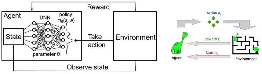
Reinforcement Learning
Spark & Databricks
Apache Spark & Databricks
Apache Spark™ is a fast and general engine for large-scale data processing.Run programs up to 100x faster than Hadoop MapReduce in memory, or 10x faster on disk.Write applications quickly in Java, Scala, Python, R.Combine SQL, streaming, and complex analytics.Spark runs on Hadoop, Mesos, standalone, or in the cloud. It can access diverse data sources including HDFS, Cassandra, HBase, and S3.
Building a Recommendation Engine
- Collaborative filtering for recommendations with Spark
- Collaborative filtering for recommendations with Spark
- Using Spark MLlib's Alternating Least Squares algorithm to make movie recommendations
- Testing the results of the recommendations
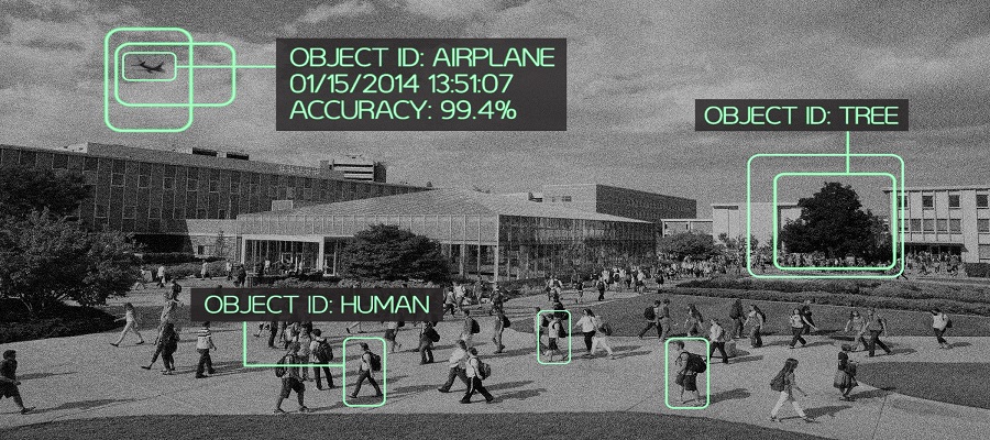
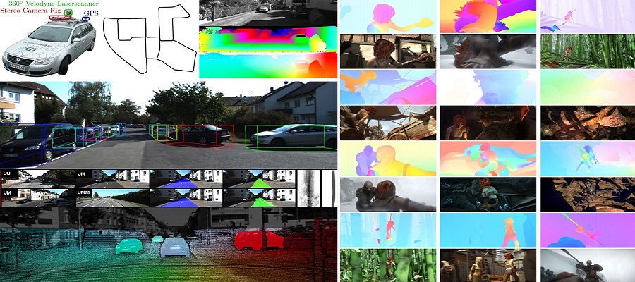
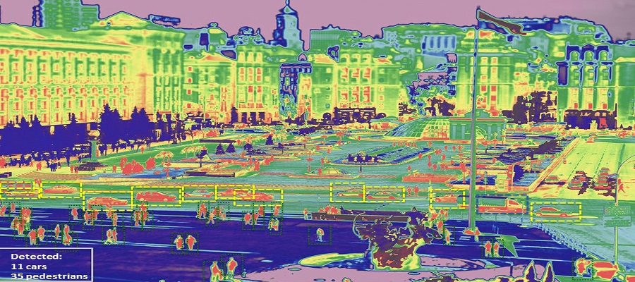
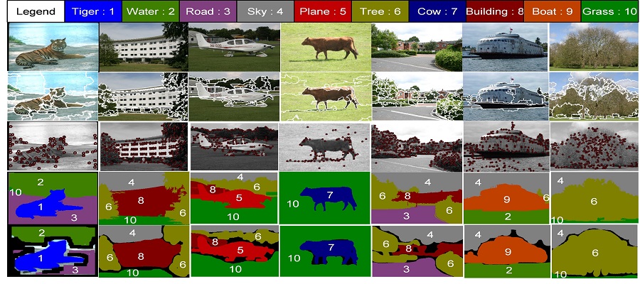
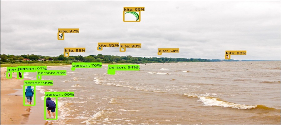
Computer Vision
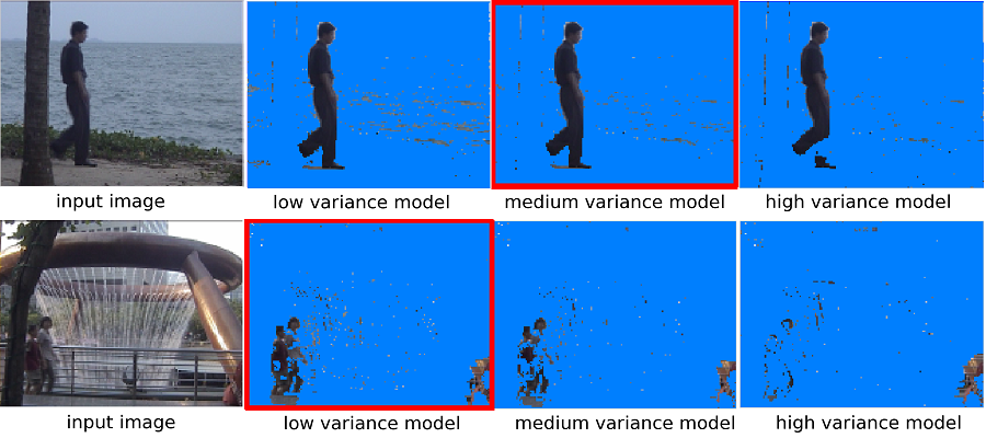
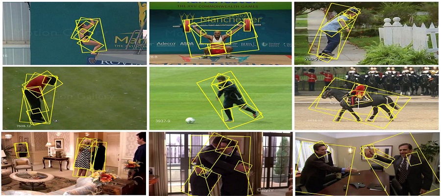

Machine Learning
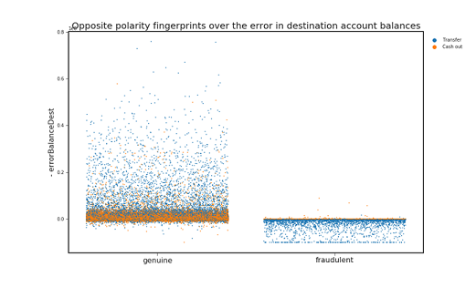
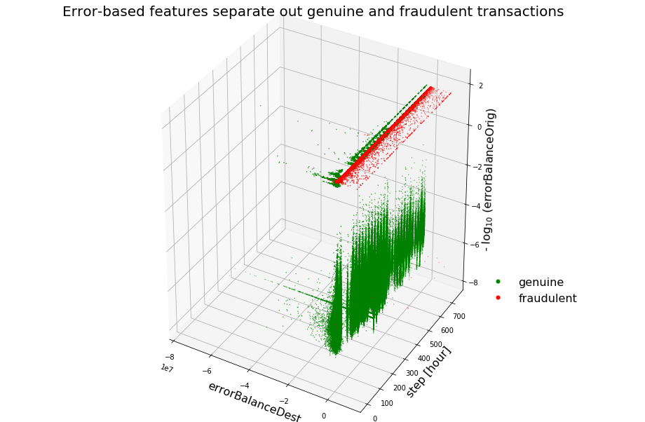
Fraud Analysis
Identify fraudulent credit card transactions.It is important that credit card companies are able to recognize fraudulent credit card transactions so that customers are not charged for items that they did not purchase.
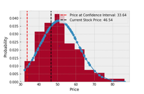
Histogram of speculated stock price
Monte Carlo simulation of a stock price is random. A histogram is plotted which shows the probability distribution of the random stock prices, so as to get an estimate of how the stock price may take on different values in the future. It is also useful for comparison with current stock price as shown in the figure.
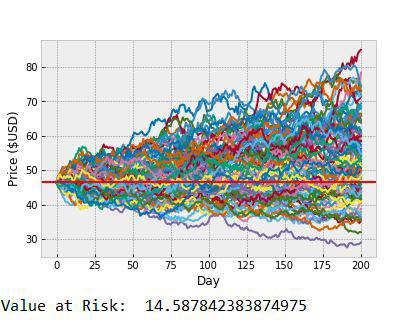
Monte carlo simulation : 200 Days
Monte carlo simulation has been performed 100 times for 200 days from the last available date in the dataset. The plot for the 100 simulations for 200 days has been shown in the adjacent figure. We can also see the current stock price and so get an idea of how the price may vary over the next 200 days Value at risk (VaR) is used to measure and quantify the level of financial risk within a firm or investment portfolio over a specific time frame. This can be estimated as part of Monte Carlo simulation as can be seen in the adjacent figure.
Entertainment
Our Platform allows digital advertisers to analyze the massive amount of personal data that consumers share, and offer those consumers more personalized and targeted ads for products and services they would use. It can also provide advertising companies with the ability to seamlessly run a real-time automated advertising platform.
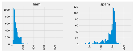
Spam and Ham Detection
Identify particular message as Ham/Spam from various sources(Emails, Text Document, Reviews etc…).
Tableaq
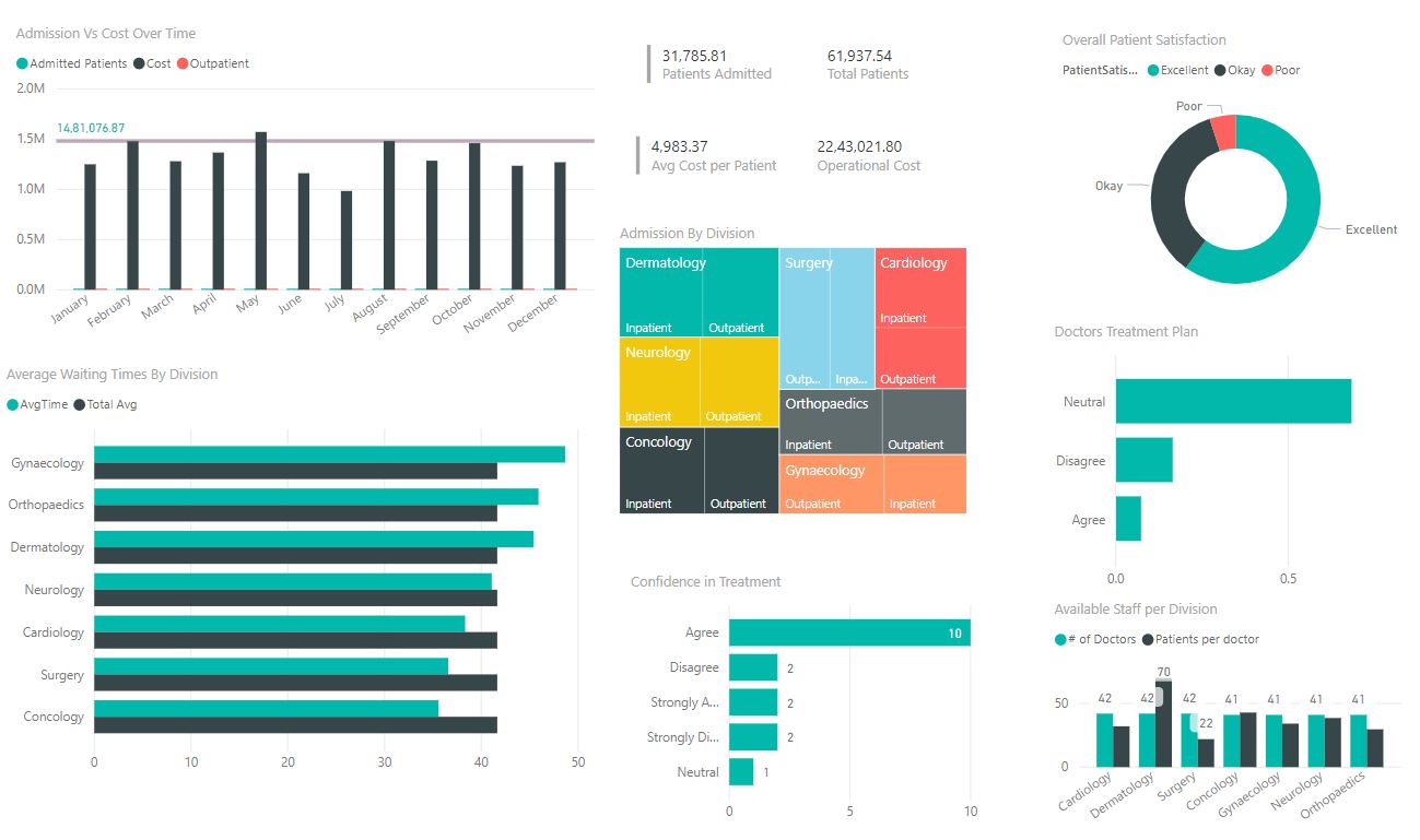
Hospital/Patient Analytics
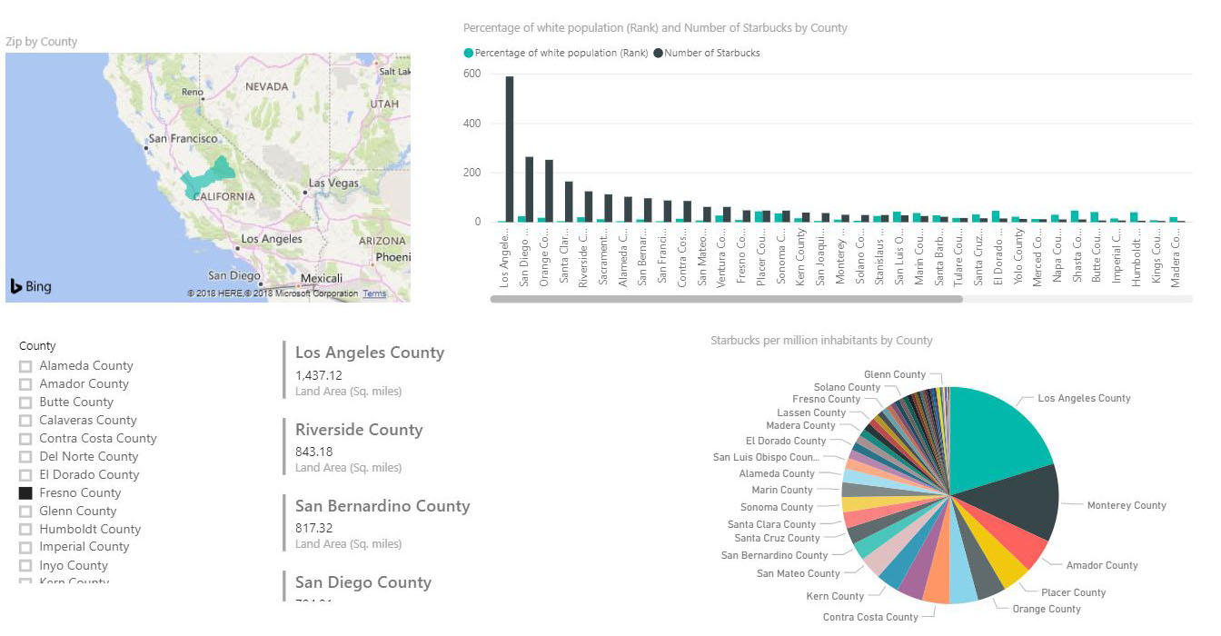
Starbucks Inhabitants Dashboard
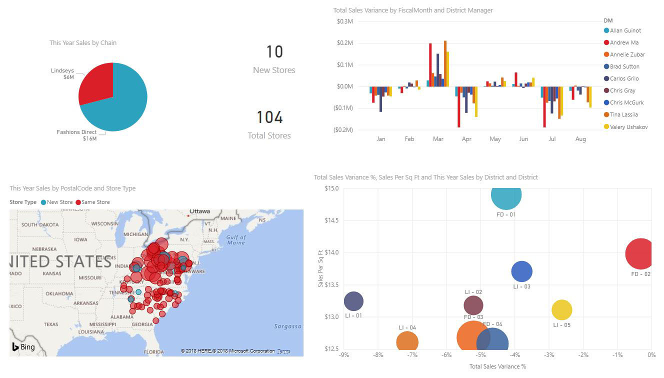
Store Sales Overview
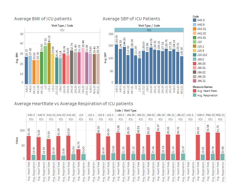
ICU Patient Analysis
Splunk
Docker & Kubernetes
Containers are great to use to make sure that your analyses and models are
reproducible across different environments. While containers are useful for keeping dependencies
clean on a single machine, the main benefit is that they enable data scientists to write model
endpoints without worrying about how the container will be hosted. This separation of concerns makes
it easier to partner with engineering teams to deploy models to production, or using the approaches
shown in this chapter data and applied science teams can also own the deployment of models to
production.
The best approach to use for serving models depends on your deployment environment and expected
workload. Typically, you are constrained to a specific cloud platform when working at a company,
because your model service may need to interface with other components in the cloud, such as a
database or cloud storage. Within AWS, there are multiple options for hosting containers while GCP
is aligned on GKE as a single solution.
The main question to ask is whether it is more cost effective to serve your model using serverless
function technologies or elastic container technologies. The correct answer will depend on the
volume of traffic you need to handle, the amount of latency that is tolerable for end users, and the
complexity of models that you need to host. Containerized solutions are great for serving complex
models and making sure that you can meet latency requirements, but may require a bit more DevOps
overhead versus serverless functions.
Python
- Web Applications
- Machine Learning, Deep Learning, Computer Vision etc..
- Bigdata, Spark and Hadoop
- Application Development
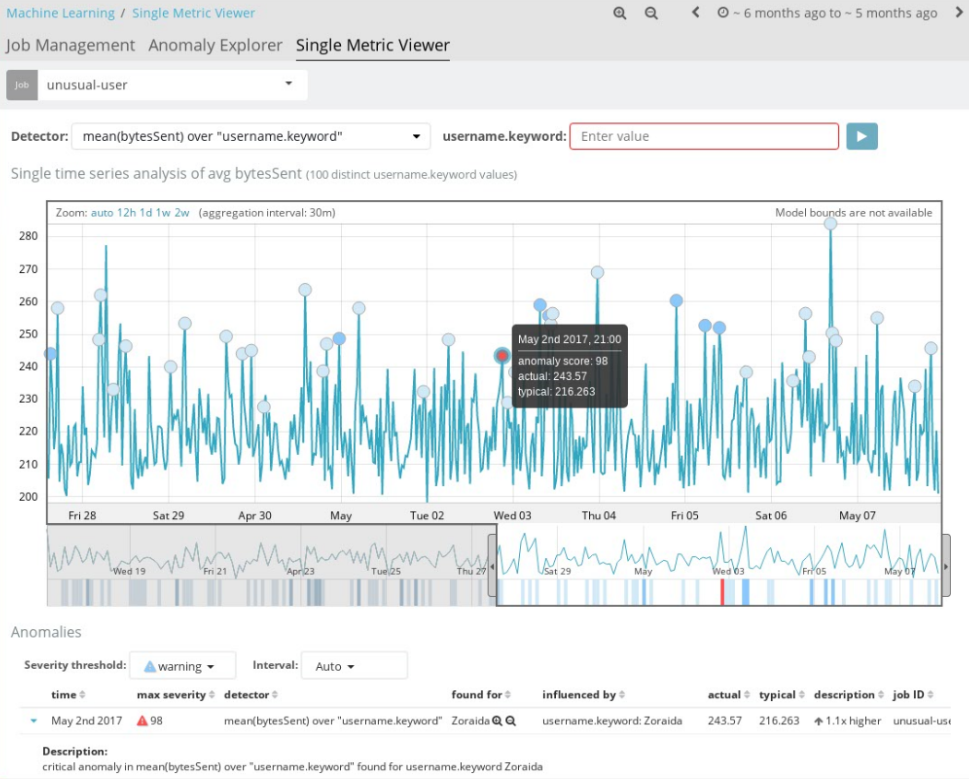
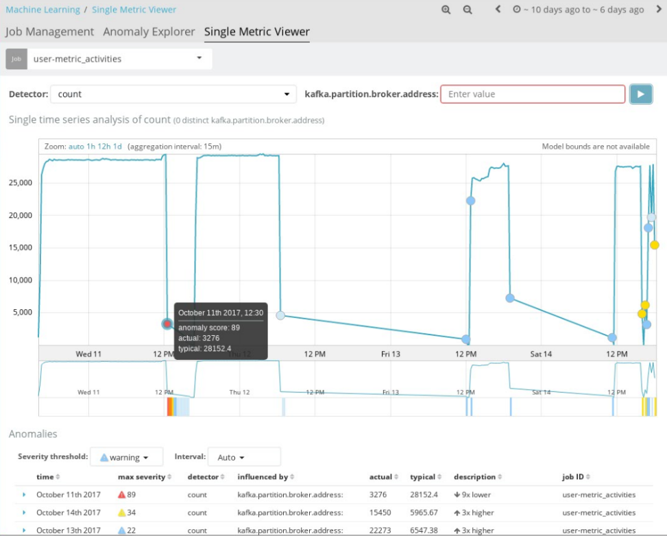
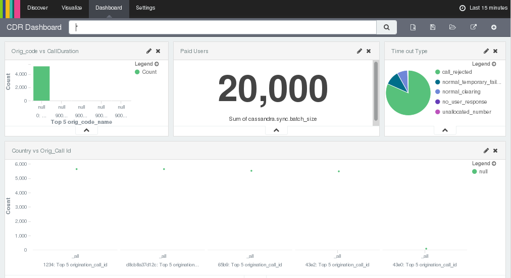
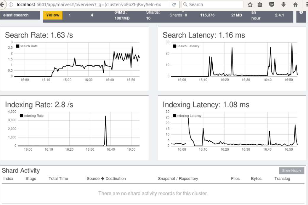
Elastic Search
Data Migration to NoSQL Databases
Migrate data from Relational Databases (Oracle/MySQL etc..) to ElasticSearch etc....
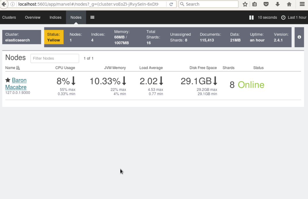
ElasticStack(ElasticSearch) Dashboards
Elasticsearch is a distributed, RESTful search and analytics engine capable of solving a growing number of use cases. As the heart of the Elastic Stack, it centrally stores your data so you can discover the expected and uncover the unexpected.
Nifi
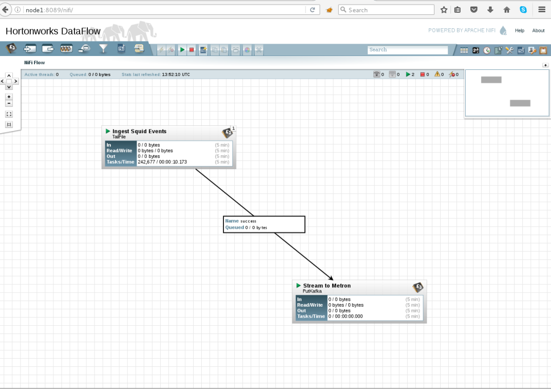
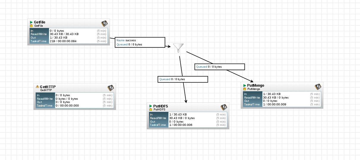
Apache Nifi
An easy to use, powerful, and reliable system to process and distribute data.Apache NiFi supports powerful and scalable directed graphs of data routing, transformation, and system mediation logic. Some of the high-level capabilities and objectives of Apache NiFi include: * Web-based user interface * Highly configurable * Data Provenance * Designed for extension * Secure.
Mean Stack
MEAN Stack Application Development
Empower your application’s efficiency with power-packed JavaScript based technologies Streamline your application with MEAN stack development
MEAN Stack is essentially a software bundle that can help developers build hybrid apps that are
extremely efficient in the shortest amount of time. MEAN is an acronym for the four software used to
build your website or app, they are MongoDB, Express.js, AngularJS and Node.js, together they create
a powerhouse of platforms that some of the best developers at GoodWorkLabs use to create the fastest
and sleekest applications and websites on the market.
The four platforms put together help create an environment that is has beautifully and
efficiently designed front end and back end, synced to perfection, and stored in a database that
vastly improves the functionality of your website or app. And all that done in a fraction of the
lines of code usual developers would have to write. If you happen to be looking for the above
mentioned advantages, then your search stops now. GoodWorkLabs is simply the Best MEAN Stack
Development Company you will ever find.
Scale up your business to a whole new level by our Mean Stack Development Services
Microsoft AI/ML and Dynamics
Microsoft Cognitive Services
Use AI to solve business problems
- Vision Image-processing algorithms to smartly identify, caption, index, and moderate your pictures and videos.
- Speech Convert spoken audio into text, use voice for verification, or add speaker recognition to your app.
- Knowledge Map complex information and data in order to solve tasks such as intelligent recommendations and semantic search.
- Search Add Bing Search APIs to your apps and harness the ability to comb billions of webpages, images, videos, and news with a single API call.
- LanguageAllow your apps to process natural language with pre-built scripts, evaluate sentiment and learn how to recognize what users want.
Microsoft Dynamics AX/2012/365
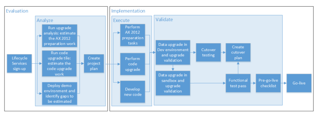
Microsoft just made a great affordable solution even better! 2017 will see the end of mainstream support for Dynamics CRM 4.0 and CRM 2011. And what better time to upgrade and experience the fantastic new features from Dynamics 365, to streamline your business processes. If you are still on an older version, the upgrade will not only be a tremendous face-lift, but alongside brings you the power of data and cloud to draw insights which you didn’t even know existed.
Upgrade to Microsoft Dynamics 365
Deep Learning
Deep Learning has enabled many practical applications of Machine Learning and by extension the overall field of AI. Deep Learning breaks down tasks in ways that makes all kinds of machine assists seem possible, even likely. Driverless cars, better preventive healthcare, even better movie recommendations, are all here today or on the horizon. AI is the present and the future. With Deep Learning’s help, AI may even get to that science fiction state we’ve so long imagined.
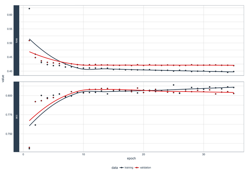
Deep Learning Training Results
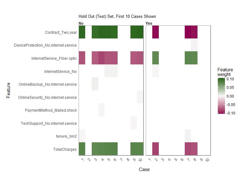
Lime Feature Importance Heatmap
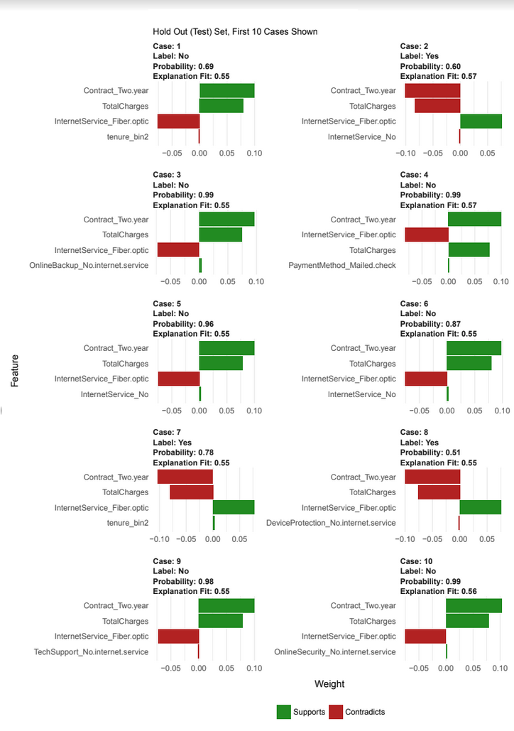
Lime Feature Importance Visualizations
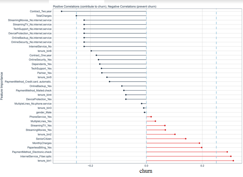
Churn Correlation Analysis
IBM Cognos TM1/BI
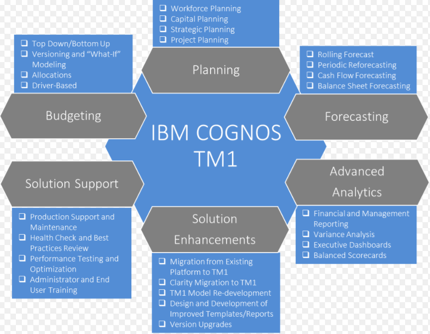
IBM Cognos TM1 is an enterprise planning software platform that can transform your entire planning cycle, from target setting and budgeting to reporting, scorecarding, analysis and forecasting. Available as an on-premise or on-cloud solution, and with extensive mobile capabilities, IBM Cognos TM1 enables you to collaborate on plans, budgets and forecasts.
Planning, Budgeting and Forecasting using IBM Cognos BI & TM1
R
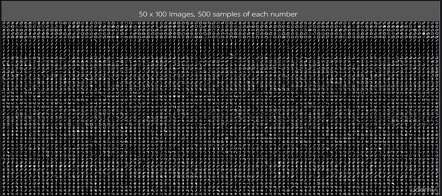
Convolutional Neural Networks:
# Clean workspace
                            rm(list=ls())
                            setwd("D:/MyOne/R/R programes/ppts/cse 7219/cnn")

                            # Installation of mxnet library
                            #install.packages("drat", repos="http://cran.rstudio.com")
                            #drat:::addRepo("dmlc")
                            #install.packages("mxnet")


                            cran <- getOption("repos")
                            cran["dmlc"] <- "https://s3.amazonaws.com/mxnet-r/"
                            options(repos = cran)
                            #install.packages("mxnet")
                            # Load MXNet
                            require(mxnet)
                            library(mxnet)

                            # Loading data and set up

                            # Load train and test datasets
                            train <- read.csv("train_sample.csv")
                            test <- read.csv("test_sample.csv")

                            ###########################################
                            ###########################################  Viewing the Images ########################
                            train_mat <- as.matrix(train)
                            # inc <- which(results_test[,3] == 0)

                            ## Color ramp def.
                            colors <- c('white','black')
                            cus_col <- colorRampPalette(colors=colors)

                            ## Plot the first 12 images
                            par(mfrow=c(4,3),pty='s',mar=c(1,1,1,1),xaxt='n',yaxt='n')
                            sm = sample(nrow(train_mat), 12)
                            for(di in sm)
                            {
                              print(di)
                              #   all_img[di+1,] <- apply(train[train[,785]==di,-785],2,sum)
                              #   all_img[di+1,] <- all_img[di+1,]/max(all_img[di+1,])*255

                              z <- array(train_mat[di,-1],dim=c(28,28))
                              z <- z[,28:1] ##right side up
                              z <- matrix(as.numeric(z), 28, 28)
                              image(1:28,1:28,z,main=train_mat[di,1],col=cus_col(256))
                            }
                            ##############################################################################
                            ###########################################  Dat Preprocessing in required format for mxnet library ###########
                            # In our actual data, first column is target attribute and other columns represent the attributes
                            # each row represents a record/sample/imge
                            # In mxnet library each column represents the record and each row reprsents an attribute and hence
                            # taking transpose of our actual data to make it compatible to the mxnet.
                            # Actually each row represents an image - it is in a vector format.  We need to convert this into 2D matrix
                            # to represent the image  28 * 28 matrix - 784 values represent each image
                            # first column is the target attribute and hence remove this and remaining 784 cells will become the data for each imge
                            # train_x is the transpose of train data .
                            # in train_x, columns are the number of images/samples.  similaryly test_x
                            ##############################################################################

                            # Set up train and test datasets
                            train <- data.matrix(train)
                            train_x <- t(train[, -1])
                            train_y <- train[, 1]
                            train_array <- train_x
                            dim(train_array) <- c(28, 28, 1, ncol(train_x))

                            test_x <- t(test[, -1])
                            test_y <- test[, 1]
                            test_array <- test_x
                            dim(test_array) <- c(28, 28, 1, ncol(test_x))

                            # Set up the symbolic model
                            # creating the variable data in mxnet format
                            data <- mx.symbol.Variable('data')

                            # kernel represnets the size of kernel and num_filter represents the number of kernels
                            # act_type is the activation function
                            # stride is the size with which the kernel shape (to shift on data matrix)

                            # 1st convolutional layer  5x5 kernel and 16 filters
                            conv_1 <- mx.symbol.Convolution(data = data, kernel = c(5, 5), num_filter = 16)
                            relu_1 <- mx.symbol.Activation(data = conv_1, act_type = "relu")
                            pool_1 <- mx.symbol.Pooling(data = relu_1, pool_type = "max", kernel = c(2, 2),
                                                        stride = c(2, 2))


                            # 2nd convolutional layer 5x5 kernel and 32 filters
                            conv_2 <- mx.symbol.Convolution(data = pool_1, kernel = c(5, 5), num_filter = 32)
                            relu_2 <- mx.symbol.Activation(data = conv_2, act_type = "relu")
                            pool_2 <- mx.symbol.Pooling(data=relu_2, pool_type = "max", kernel = c(2, 2),
                                                        stride = c(2, 2))


                            # 1st fully connected layer (Input & Hidden layers)
                            flatten <- mx.symbol.Flatten(data = pool_2)
                            fc_1 <- mx.symbol.FullyConnected(data = flatten, num_hidden = 128)
                            relu_3 <- mx.symbol.Activation(data = fc_1, act_type = "relu")


                            # 2nd fully connected layer(Hidden & Output layers)
                            # num_hidden here is the number of target class levels
                            fc_2 <- mx.symbol.FullyConnected(data = relu_3, num_hidden = 10)
                            # Output. Softmax output since we'd like to get some probabilities.
                            NN_model <- mx.symbol.SoftmaxOutput(data = fc_2)

                            # Pre-training set up

                            # Set seed for reproducibility
                            mx.set.seed(100)

                            # Create a mxnet CPU context. - Device used. CPU in this case, but not the GPU
                            devices <- mx.cpu()

                            # Training


                            # Train the model
                            model <- mx.model.FeedForward.create(NN_model,
                                                                 X = train_array,
                                                                 y = train_y,
                                                                 ctx = devices,
                                                                 num.round = 20, # number of epochs
                                                                 array.batch.size = 40,
                                                                 learning.rate = 0.01,
                                                                 momentum = 0.5,
                                                                 eval.metric = mx.metric.accuracy,
                                                                 epoch.end.callback = mx.callback.log.train.metric(100))

                            # Testing

                            # Predict labels
                            predicted <- predict(model, test_array)
                            # Assign labels
                            predicted_labels <- max.col(t(predicted)) - 1
                            # Get accuracy
                            (sum(diag(table(test[, 1], predicted_labels)))/1000) * 100
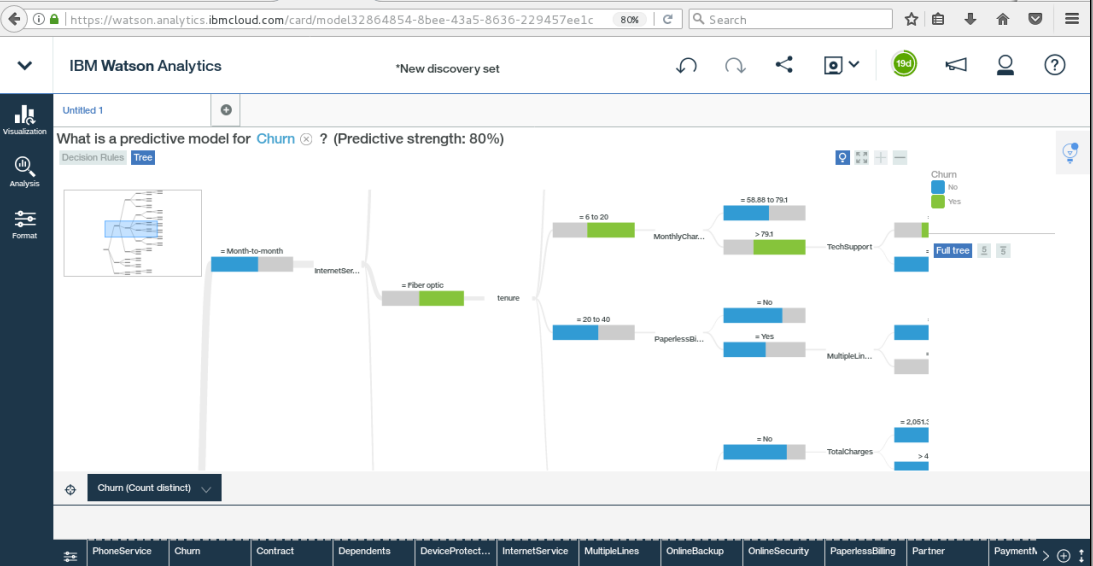
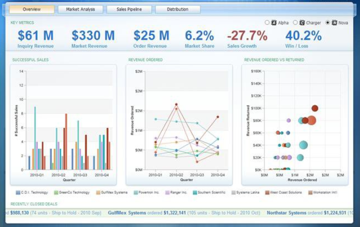
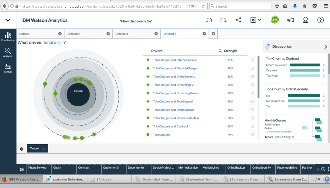
Watson Analytics
IBM Watson Analytics is a cloud-based data discovery service intended to provide the benefits of advanced analytics without the complexity. Here are eight organizations using Watson Analytics to transform their operations.
Tenure Discovery
Profit Dashboard
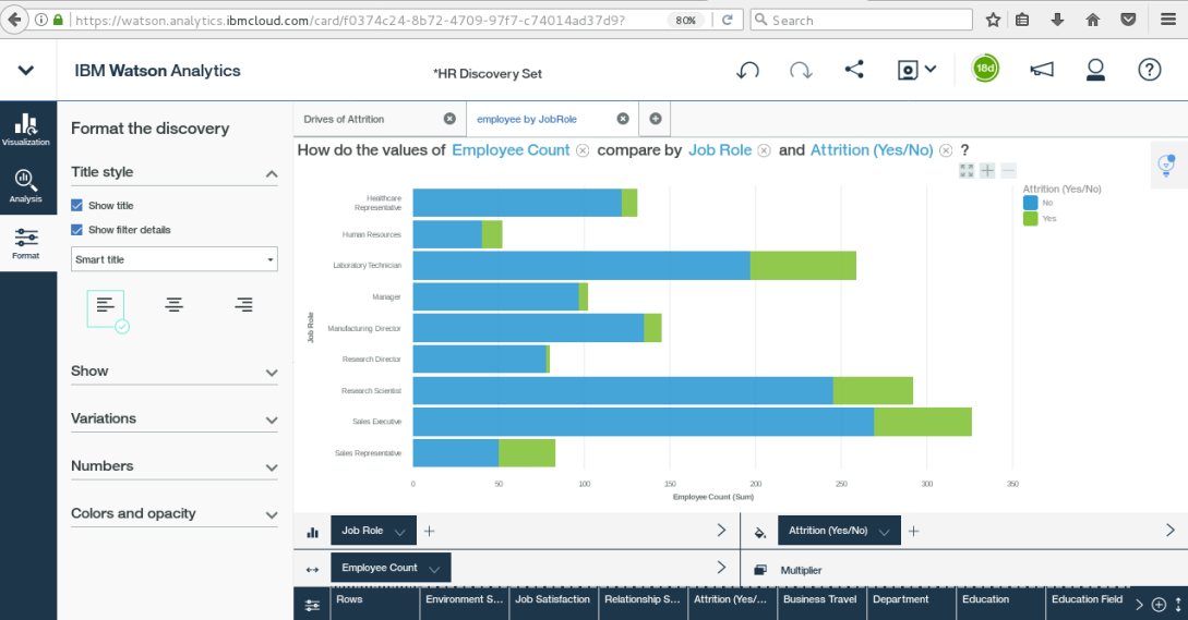
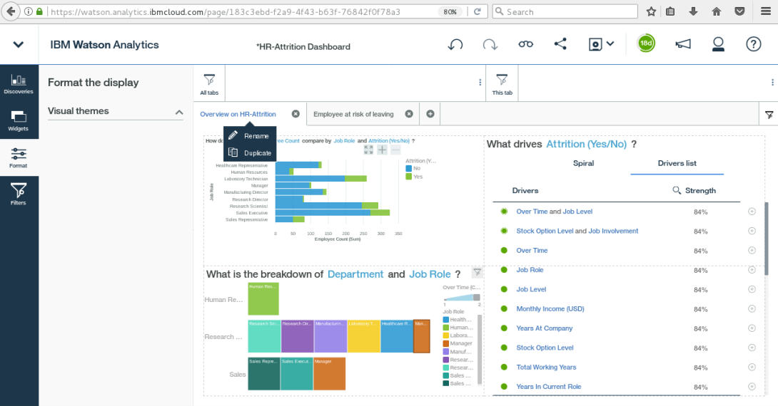
HR Attrition
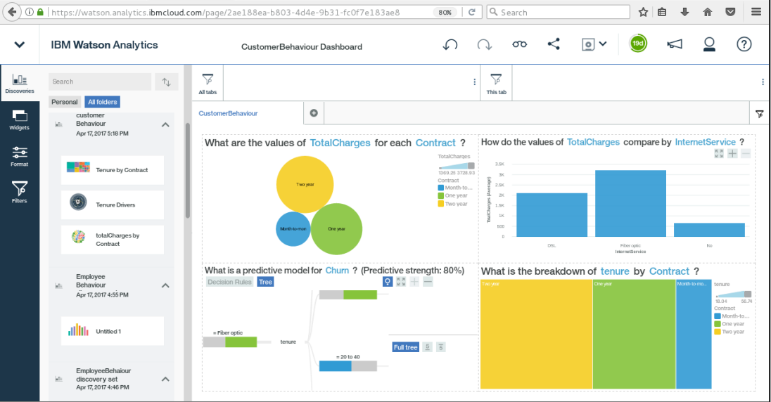
Customer Behaviour
Churn Prediction